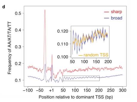
The autors classified promoters based on their initiation pattern into
two classes: broad and sharp. They then studied the base composition
around them. They found a characteristic signal in the region +50 to
+200 bp from the TSS that show a strong periodic signal. This signal
is similar to the one from MNase-seq experiments of region with high
nucleosome affinity.
Hints and recipes
Note that the data used in this paper is present on the ChIP-Seq
server, aligned on hg19 genome assembly.
To reproduce the figures you should:
-
First classify promoters based on their initiation patterns. To do
so, use CAGE data from the ENCODE consortium (all samples
cell longPolyA).
-
To do so you have first to extract CAGE data around EPDnew
promoters using ChIP-Extract. Use EPDnew 003 for hg19 as
reference feature (oriented) and ENCODE CAGE data (all samples
cell longPolyA) as target feature (only the plus
strand). Select a range from -100 to 100, Window width 1 and
count cut-off 9999999.
-
Run the job and save the sga file as "promoters.sga" and the
TEXT file as "promoters_expression.out".
-
Now evaluate promoter initiation pattern in R. Peak promoters
have CAGE distribution very close to the TSS whereas broad
promoters have CAGE tags spread around a larger area. You can
use the Dispersion Index [Note: this is not the exact code
used by the autors, is our own method but should provide
similar results] in R using the following code:
      dispersion <- function(x){

        tss <- ceiling(length(x)/2)

        region <- length(x)

        if(sum(x) == 0) {

            m <- 0

            s <- -1

        } else {

            m <- sum(x*(1:region))/sum(x)

            s <- (sum((x*(1:region-m)**2))/sum(x))**0.5

        }

        return(s)

      }


      p.expression <- read.table("promoters_expression.out")

      p.dispersion <- apply(p.expression, 1, dispersion)


      # The following read the SGA file with the promoter collection

      promoters <- read.table("promoters.sga", as.is=T)


      # The following concatenate the SGA file with the Dispersion Index

      promoters <- cbind(promoters,p.dispersion)


      # The following write out a new SGA file with 7th column as Dispersion Index

      write.table(promoters, file="promotersDispersionIndex.sga", quote=F, sep="\t", col.names=F, row.names=F)
In R check the distribution of the Dispersion Index values ad
try to set a cut-off between broad and peak promoters (peak
promoters should be 10-15% of all active promoters). [Note: some
promoters have no expression, the Dispersion Index is set to -1,
exclude those from the analysis]. To do so, you can use the
following plot:
plot(density(p.dispersion), type="l")
-
Use a cut-off value of 12 to group promoters using the following code:
peak <- which(p.dispersion > 0 & p.dispersion < 12)

broad <- which(p.dispersion >= 12)


write.table(promoters[peak,], file="peakPromoters.sga", quote=F, sep="\t", col.names=F, row.names=F)

write.table(promoters[broad,], file="broadPromoters.sga", quote=F, sep="\t", col.names=F, row.names=F)
-
In your working directory you have two SGA file:
"peakPromoters.sga" and "broadPromoters.sga" that you will now
analyse for the presence of nucleosome signal.
-
Convert final SGA files in FPS using ChIP-Convert tool (the SSA
server that we have to use next only accepts FPS file format).
-
Study dinucleotide frequencies around promoters using OProf tool
from SSA. The autors used WW (W = A or T), but these are not the
only dinucleotides that are know to have high nucleosome
affinity. Try also SS (S = G or T), YY (Y = C or T) and RR (R = A
or G). To do so, do as follow:
-
Upload your files as imput FPS file
-
Extend the range of the 3' border to 300, use a window size of
3 and a shift of 1 base
-
Use WW as consensus sequence with no mismatches and reference
position 1
-
Run the job and save the text file
-
Use R to import the text files and reproduce the figure.

