Chip-seq data analysis: from quality check to motif discovery and more

Lausanne, 27 March - 31 March 2017

Data reproduction exercise: Consistency of ChIPseq replicates - analysis using IDR

Authors: Sunil Kumar and Philipp Bucher


Introduction

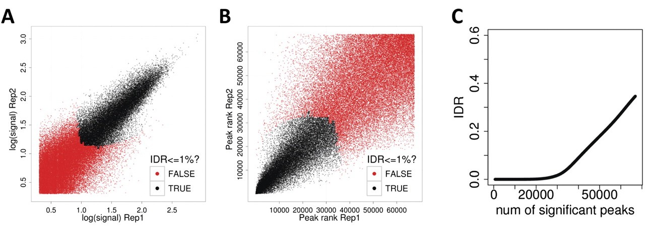
Current exercise is baesd on the following paper: The publication contain details of various good practices and guidelines followed by ENCODE and modENCODE consortia. One of the guideline deals with analyzing the reproduciility of ChIP-seq replicates. In this exercise we will try to make a figure similar to the one from the paper (Figure 6).

Reproducibility analysis for a pair of high-quality RAD21 ChIP-seq replicates. Scatter plots of A) signal scores and B) ranks of peaks that overlap in the pair of replicates. C) The estimated IDR as a function of different rank thresholds. Black data points represent pairs of peaks that pass an IDR threshold of 1%, whereas the red data points represent pairs of peaks that do not pass the IDR threshold of 1%.

Irreproducible discovery rate (IDR)

As a general rule the modENCODE and ENCODE consortia generate two independent biological replicates, with each experiment passing the basic quality control filters. As another measure of experiment quality, they check the reproducibility information from the duplicates using the irreproducible discovery rate (IDR) statistic. The method was developed by Qunhua Li and Peter Bickel's group and is extensively used by the ENCODE and modENCODE projects and is part of their ChIP-seq guidelines and standards (Li et al. 2011).

The basic idea is that if two replicates measure the same underlying biology, the most significant peaks, which are likely to be genuine signals, are expected to have high consistency between replicates, whereas peaks with low significance, which are more likely to be noise, are expected to have low consistency. If the consistency between a pair of rank lists (peaks) that contains both significant and insignificant findings is plotted, a transition in consistency is expected (Fig. 1C). This consistency transition provides an internal indicator of the change from signal to noise and suggests how many peaks have been reliably detected.

According to ENCODE consortia this IDR pipeline is extensively tested and verified for human transcription factor ChIP-seq data and punctate chromatin marks (e.g. H3k9ac, H3k27ac, H3k4me3, H3k4me1 etc.) using the SPP peak caller.

Original IDR CODE may be downloaded from: Code archive. There is also a R implementation for IDR: CRAN version. However, the CRAN package implements a slightly different underlying algorithm and is more general purpose, so the ENCODE developers recommend using their code even though it is a bit clunky.

Caution while applying IDR:

Hints and recipes

We will need atleast two replicate for any ChIPseq experiments for testing through IDR pipeline. The basic requirements are:

Example for the current exercise: download the following two files that have been taken from GEO series GSE30263 CTCF Binding Sites by ChIP-seq from ENCODE/University of Washington.
  • CTCF replicate1 from HUVEC cell line.
  • CTCF replicate2 from HUVEC cell line.

    In addition you will need to download the following files:

  • R functions: source file that contain all the functions required for IDR analysis.
  • Genome table

    Running IDR

    Please be informed that the IDR code written below is taken from the ENCODE and if you need to know more about it please refer to IDR page.

    R script for IDR Hide script

    Navigate into the directory containing data and launch R. Load the following file:

      source("functions-all-clayton-12-13.R")

    Read peak files and genome table:

      peakfile1 <- "HUVEC_hg19_CTCF_rep1.bed"
      peakfile2 <- "HUVEC_hg19_CTCF_rep2.bed"
      
      chr.size <- read.table("genome_table.txt")
      
    Define parameters:
      half.width <- NULL
      overlap.ratio <- 0
      is.broadpeak <- F
      sig.value <- "p.value"
      

    • [half.width]: Set this to -1 (NULL) if you want to use the reported peak width in the peak files.
    • [overlap.ratio]: fractional bp overlap (ranges from 0 to 1) between peaks in replicates to be considered as overlapping peaks. IMPORTANT: This parameter has not been tested fully. It is recommended to set this to 0.
    • [is.broadpeak]: Is the peak file format narrowPeak or broadPeak. Set to F if it is narrowPeak/regionPeak or T if it is broadPeak.
    • [ranking.measure] is the ranking measure to use. It can take only one of the following values signal.value, p.value or q.value.
    Process data and generate IDR output.
      rep1 <- process.narrowpeak(paste(peakfile1, sep=""), chr.size, 
      	half.width=half.width, summit="offset", broadpeak=is.broadpeak)
      rep2 <- process.narrowpeak(paste(peakfile2, sep=""), chr.size, 
      	half.width=half.width, summit="offset", broadpeak=is.broadpeak)
      uri.output <- compute.pair.uri(rep1$data.cleaned, rep2$data.cleaned, 
      	sig.value1=sig.value, sig.value2=sig.value, overlap.ratio=overlap.ratio)
      em.output <- fit.em(uri.output$data12.enrich, fix.rho2=T)
      idr.local <- 1-em.output$em.fit$e.z
      IDR <- c()
      o <- order(idr.local)
      IDR[o] <- cumsum(idr.local[o])/c(1:length(o))
      idr_output <- data.frame(chr1=em.output$data.pruned$sample1[, "chr"],
                          start1=em.output$data.pruned$sample1[, "start.ori"],
                          stop1=em.output$data.pruned$sample1[, "stop.ori"],
                          sig.value1=em.output$data.pruned$sample1[, "sig.value"],   
                          chr2=em.output$data.pruned$sample2[, "chr"],
                          start2=em.output$data.pruned$sample2[, "start.ori"],
                          stop2=em.output$data.pruned$sample2[, "stop.ori"],
                          sig.value2=em.output$data.pruned$sample2[, "sig.value"],
                          idr.local=1-em.output$em.fit$e.z, IDR=IDR)
      
      write.table(idr_output, "idr_overlapped_peaks.txt", sep="", quote=F)
      
    Getting peaks that pass the IDR threshold:
      filtered_peaks <- idr_output[idr_output[,10]<=0.01,]
      dim(filtered_peaks) # get the number of peaks
      
    Plotting the results Hide script
      ez.list <- get.ez.tt.all(em.output, uri.output$data12.enrich$merge1, uri.output$data12.enrich$merge2)
      par(mar=c(5,5,0,0.5), mfrow = c(1,3), oma=c(5,0,2,0))
      idr_output$col[idr_output[,10]<=0.01]="black"
      idr_output$col[idr_output[,10]>=0.01]="red"
      plot(log(idr_output[,4]),log(idr_output[,8]),col=idr_output[,11], pch=19, 
      	xlab="log(signal) Rep1", ylab="log(signal) Rep2")
      legend("topleft", c("IDR=>0.01","IDR<=0.01"), col=c("red","black"), pch=19, 
      	bty="n", lty=c(1,1), lwd=c(2,2))
      plot(rank(-idr_output[,4]),rank(-idr_output[,8]),col=idr_output[,11], pch=19, 
      	xlab="Peak rank Rep1", ylab="Peak rank Rep2")
      legend("topleft", c("IDR=>0.01","IDR<=0.01"), col=c("red","black"), pch=19, 
      	  bty="n", lty=c(1,1), lwd=c(1,1))
      plot(ez.list$IDR, ylab="IDR", xlab="num of significant peaks")
      

    You can join the IDR mailing list https://groups.google.com/group/idr-discuss for FAQs, discussions and updates on software.