Peak list evaluation

Chip-seq data analysis: from quality check to motif discovery and more

Lausanne, 27 March - 31 March 2017

Data reproduction exercise: Peak list evaluation - motif enrichment test

Author: Philipp Bucher, Romain Groux

Introduction

This exercise is based on the following paper:

20628599

As the title indicates, the paper presents a performance evaluation of Chick-seq peak-finder software. The authors use various statistical plots for this purpose. Note that all these tests require as input a ranked peak list and a reference set of bona fide true binding sites.

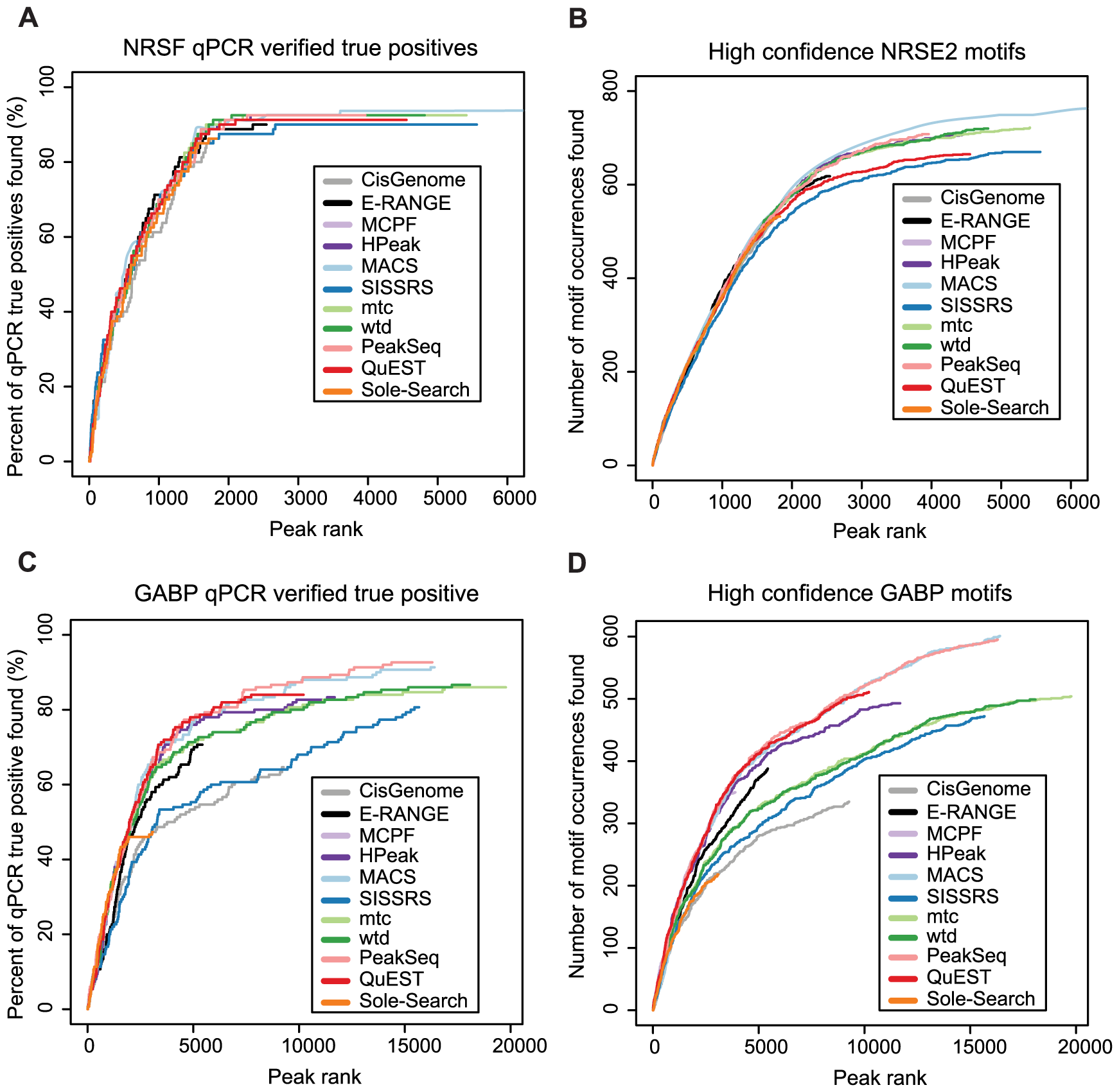
Figure 5 compares peak lists obtained with different peak finders with so-called sensitivity plots.

These plots show the total number of true positive among the N highest ranking peaks as a function of N. True positives are either defined by a given set of experimentally validated binding sites or by the presence of a binding motif of the corresponding transcription factor.

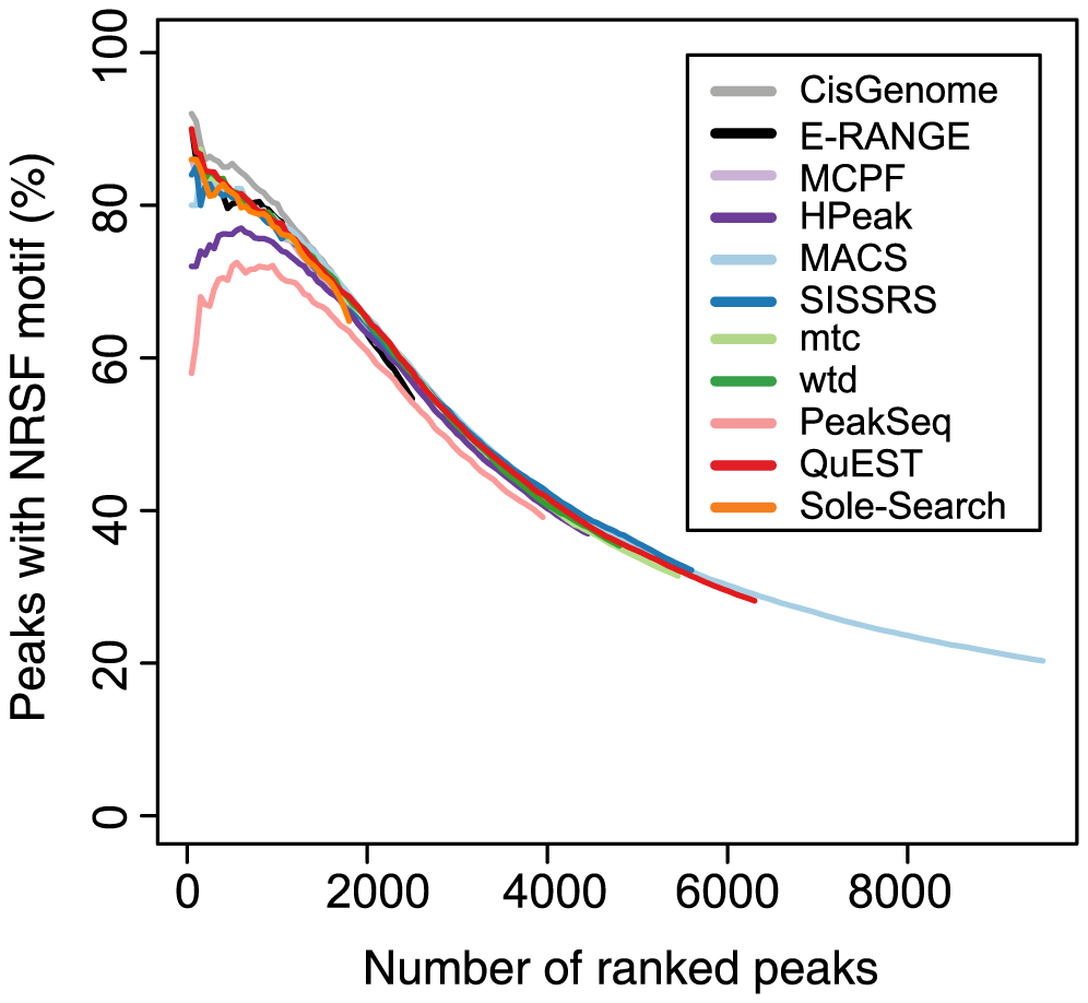
Figure 6 shows the ranking accuracy obtained with different peak finders for NRSF.

In principle, one would expect the top-ranked peaks to be the most highly enriched in the NRSF binding sites. As you can see, this is not the case for all Peak finders.

Exercise

Generate peak lists for NRSF and GABP with ChIP-Peak. Then generate sensitivity and ranking accuracy plots for the resulting peak lists. Next, compute the same types of curves for other NRSF and GABP peak lists available at our server. At the end, superpose the curves obtained with different peak lists in single graphics.

Hints and recipes

Input data

ChIP-seq and ChIP-seq-peak data from hg18:

    Valouev 2008, Jurkat cells, GABP SRF NRSF
       Sample: Jurkat GABP
       Sample: Jurkat NRSF(polyclonal)
       Sample: Jurkat NRSF(monoclonal)

Additional peak lists for GABP and NRSF from hg19 can be found in:

   ENCODE ChIP-seq-peak -> Uniform TFBS from UCSC

qPCR-validated binding site lists:

These lists are avaible in a Excel file named "Dataset S1" posted on the publisher's website under "Supporting Information". The Excel file contains two sheets, one for GABP and one for NSRF, which you have to export seperately in Text CSV format (field delimiter tab, text delimiter none). The exported files are posted below:

wilbanks_DS1_GABP.txt

wilbanks_DS1_NRSF.txt

The binding site coordinates are given for human genome assembly hg18. The above files can be converted into server-compatible BED files with R:

   GABP = read.table("wilbanks_DS1_GABP.txt")
   GABP = GABP[-1,]
   write.table(GABP[,1:3],"GABP_qPCR.bed",
      row.names=F, col.names=F, sep="\t", quote=F)

The binding site table for NRSF has an additional column filled with the enrichment factor. According to Mortazavi et al. (PMID: 16963704) only sites with enrichment values higher than 2.44 should be considered as positives. This is taken into account with the following conversion recipe.

   NRSF = read.table("wilbanks_DS1_NRSF.txt", as.is=4)
   NRSF = NRSF[-1,]
   pos=which(as.numeric(NRSF[,4]) > 2.44)
   write.table(NRSF[pos,1:3],"NRSF_qPCR.bed",
      row.names=F, col.names=F, sep="\t", quote=F)

The BED files can be uploaded to ChIP-Convert for convervsion into SGA format (Compress output off, centered SGA on, Unoriented SGA on). We recommend to liftOver the resulting files to hg19 and to save SGA files for both assemblies.

All files resulting from the conversion procedure are posted below for your convenience. We recommend to use the same file names if you do the conversion yourself.

GABP_qPCR.bed	GABP_qPCR_hg18.sga	GABP_qPCR_hg19.sga
NRSF_qPCR.bed	NRSF_qPCR_hg18.sga	NRSF_qPCR_hg19.sga

Finding peaks with ChIP-peak.

Use the standard procedure proposed in the tutorial of day one. The peak lists below

GABP_ChIP-Peak_hg18.sga

NRSFpoly_ChIP-Peak_hg18.sga

were both obtained with the following parameters.

   strand:        any   Window Width :  200   Count Cut-off:          1
   centering:      50   Vicinity Range: 200   Refine Peak Positions: on
   Repeat Masker: off   Peak Threshold:  10

Making sensitivity plots with qPCR-validated binding sites

Go to ChIP-Cor. Upload a peak list as reference feature and the corresponding qPCR-validated binding site list as target feature and set the parameters as follows:

   strand:         any   strand: any
   Count Cut-off:  999
   Beginning:     -300
   End:           -300   
   Window Width:    10

The high cut-off value preserves the numbers in the count field which will later be used for peak ranking. On ChIP-cor result page, use the "Enriched Feature Extraction Option" to annotate the ChIP-Seq peak list for colocalization with the qPCR-based binding site list with the following parameters:

   From:                                  -250
   To:                                    +250   
   Threshold:                                0
   Cut-off                                 999
   Switch to Depleted Feature Selection    off
   Ref Feature Oriented                    off

The resulting annotated peak files are posted below:

GABP_ChIP-Peak_qPCR.sga

NRSFpoly_ChIP-Peak_qPCR.sga

The PCR-validation status is indicated in the sixth field, see the following example lines.

   NC_000001.9   ChIP_R   110751869   0   17   0
   NC_000001.9   ChIP_R   110887050   0   66   1
   NC_000001.9   ChIP_R   110960004   0   10   0

the R code for making the sensitivity plots is shown below:

# computing the sensitivity curve

table=read.table("GABP_ChIP-Peak_qPCR.sga",as.is=5)
# in case a peaks is near several qPCR peaks (not likely at all)
# sets the count to 1 (acts as a boolean flag)
table[table[,6] > 0, 6] = 1
rank = order(table[,5], decreasing=T)
table=table[rank,]
N=dim(table)[1]; x = 1:N
y = rep(0,N); y[1]=table[1,6]
for(i in 2:N) {y[i]=y[i-1]+table[i,6]}

# making the figure

tot=150 # number of PCR-verified sites: 150 for GABP, 83 for NRSF
par(cex=1.2)
plot(x,100*(y/tot),t="l", col="red", ylim=c(0.0,100), xlim=c(0,20000),
   xlab="Peak rank",
   ylab="Percent of qPCR true positives found (%)")
legend("bottomright", legend=c("ChIP-Peak(t=10)"),
   lty=1, col=c("red"), bty="n")

You can now generate sensitivity plots for other GABP peaks list provided by the ENCODE consortium in the same way. Keep in mind that in the peak lists provided as serverr-resident files, the peak ranking score is given in the sixth rather than fifth field. Once you have computed all curves, you can superpose them in one Figure. This will tell you how well ChIP-peak performs as compared to the peak finders that were used for generating the published peak lists.

Making sensitivity plots based on motif enrichment

You can do this in two alternative ways, one using FindM and the other one using PWMScan. We will present the recipe based on PWMScan.

Open the PWMScan input form. Perform a whole hg18 genome scan using the following parameters:

   Genome Assemblies:    H.sapiens (March 2006 NCBI36/hg18)
   Motif Library:              JASPAR CORE 2014 vertebrates
   Motif:                                    MA0062.2 GABPA
   Bg base composition               0.29, 0.21, 0.21, 0.29
   Cut-off P-value:                                 0.00001     
   Search Strand:                                      both
   Non-overlapping matches:                         checked
   Reference position                                     0

Note that the authors of the paper use 10^-7 as P-value cut-off. This seems to low. However, they used a different program called FIMO to search for PWM matches, and P-values computed by different programs may not be comparable.

GABP_motifs_hg18.sga

For NRSF, use the JASPAR matrix named "MA0138.2 REST" (REST is a a synomym of NRSF) and save the match list under the name:

NRSF_motifs_hg18.sga

From here you can essentially follow the previous recipe for making the sensitivity plots for qPCR-validated binding sites. The next step will be to generate peak lists with motif status annotations using ChIP-Cor with the "Enriched Feature Extraction Option". Annotated peak lists are posted below for your convenience. If you are working with hg19, we provide pre-computed motif instance lists for ChIP-Cor and ChIP-extract in the sequence derived series.

GABP_ChIP-Peak_motifs.sga

NRSFpoly_ChIP-Peak_motifs.sga

Ranking accuracy plots

Ranking accuracy plots of the kind shown in Figure 6 of the paper can be generated with the following R recipe:

# computing the ranking accuracy curve

table=read.table("NRSFpoly_ChIP-Peak_motifs.sga",as.is=5)
# in case a peaks is near several motif instances (happens)
# sets the count to 1 (acts as a boolean flag)
table[table[,6] > 0, 6] = 1
rank = order(table[,5], decreasing=T)
table=table[rank,]
N=dim(table)[1]; 
x=seq(50,N-50,50)
y=x; for(i in 1:length(x)) {y[i]=sum(table[1:x[i],6])}

# making the figure

par(cex=1.2)
plot(x,100*y/x,t="l", col="red", ylim=c(0.0,100), xlim=c(0,9000),
   xlab="Number of ranked peaks",
   ylab="Percent with NRSF motif (%)")
legend("topright", legend=c("ChIP-Peak(t=10)"),
   lty=1, col=c("red"), bty="n")