PWMTools - Position Weight Matrix (PWM) model generation and evaluation

Background

The tool is used to evaluate the performance of PWM models using HT-SELEX or HT-SELEX-like data.

SELEX uses purified proteins to select high-affinity binding sites from random libraries in vitro. By utilizing new sequencing technologies it is possible to derive binding energy profiles from SELEX methods quite efficiently using a method called high-throughput SELEX (HT-SELEX). HT-SELEX consists of several cycles of incubating the DNA-binding protein with a mixture of DNA sequences, enrichment of the bound DNA sequences, sequencing a sample of them and feeding them to the next cycle. An advantage of this approach is that the output (the number of counts observed for each sequence) is digital and there is a sufficient depth of data to allow use of sophisticated staistical methods that provide more accurate models of protein DNA-binding specificity than previously available.

SMiLE-seq is a new technique for the characterization of DNA-binding proteins in a much faster, more accurate and efficient way. The core of SMiLE-seq is a microfluidic platform that involves capillary loading of in vitro-transcribed and -translated bait TFs, and target double-stranded DNA from a pool of random sequences. The transcription factor (TF) is bound to the surface of the microluidic device by antibodies and some fraction of the DNA binds to the TF. The unbound DNA is expelled by washing, so the bound fraction can be measured. Bound DNA is subjected to high-throughput sequencing and a hidden Markov model (HMM)-based TF motif discovery pipeline for de novo identification of DNA-binding specificities and affinities of different families of full-length TFs and TF dimers.

For each sequence, the sum occupancy score is calculated, which is the sum over all motif matches weighted by their respective scores. The sum occupancy score is used to rank all sequences.

Shuffled sequences are used as the negative set.

By default, the top-ranked 50% of the sequences are used for testing the PWM model.
The PWM format used is the letter-probability matrix.
For probe sequence s and matrix PWM of length k, the sum occupancy score is computed as follows:

(1)

where PWM_i(s) is the probability of base s in position i of the PWM, and p_i is the nucleotide prior (or background) probability. PWM frequencies are normalized by the background sequence composition.

The background composition normalization can be computed by the following three methods:

based on a uniform background sequence composition (uniform i.e: 0.25);
based on the nucleotide composition of the entire sequence library (library comp);
based on the nucleotide composition of each single sequence (sequence-based).

Scores of binding predictions are reported in AUC of the receiver operating characteristic curve (ROC).

The motif libraries have been downloaded from the MEME Motif Database, and include the following sets: JASPAR CORE 2018, Human and Mouse HT-SELEX motifs (Jolma 2013), UniPROBE Mouse, and HOCOMOCO (version 11).

1.1 Conversion of position frequency or count matrix (PFM, JASPAR, TRASFAC) to letter probability matrix (LPM)

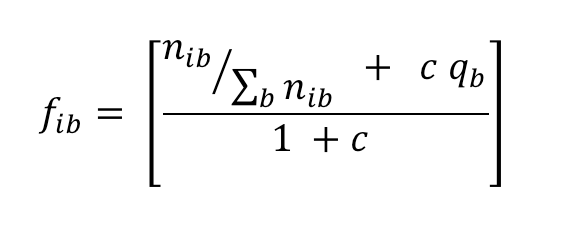
The conversion of base counts to corrected frequencies (f_i_b), that is relative frequencies which are corrected by pseudo-count fractions distributed according to residue priors, uses the following formula:

(2)

where n_i_b is the occurrences of base b at PWM position i, q_b is the background frequency of base b, and c is the fraction of pseudo-counts added to the observed base frequencies.

1.2 Conversion of position weight matrix (PWM) to letter probability matrix (LPM)

A position weight matrix can be converted to a letter probability matrix in two ways:

by using a cut-off value and a given background base composition, we generate all nucleotide sequences represented by the weight matrix and the cut-off and compute the base frequencies,
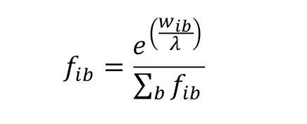
or by inverting the log likelihoods with the following formula:

(3)

where f_i_b is the probability of base b in position i of the PWM, ω_i_b the corresponding PWM weight, and λ the logarithm scaling factor used in original conversion formula to log likelihoods. So, under this assumption, we need to provide λ in order to convert the weights of the PWM to base frequencies.

Matrix Formats

TRANSFAC-style matrices look like this:

AC   M00223
XX
ID   V$STAT_01
XX
DT   29.11.1995 (created); ewi.
DT   11.03.2003 (updated); dtc.
CO   Copyright (C), Biobase GmbH.
XX
NA   STATx
XX
DE   signal transducers and activators of transcription
XX
BF   T01575 STAT1alpha; Species: mouse, Mus musculus.
BF   T01492 STAT1alpha; Species: human, Homo sapiens.
BF   T01573 STAT1beta; Species: human, Homo sapiens.
XX
PO      A      C      G      T
01      0      0      0     14      T
02      0      0      0     14      T
03      2     12      0      0      C
04      0     12      0      2      C
05      0      9      2      3      C
06      4      2      8      0      G
07      0      0      8      6      K
08     13      1      0      0      A
09     14      0      0      0      A
XX
BA   14 genomic sequences of 14 different genes
XX
CC   compiled sequences
XX
RN   [1]; RE0003481.
RX   PUBMED: 7774815.
RA   Horvath C. M., Wen Z., Darnell jr J. E.
RT   A STAT protein domain that determines DNA sequence recognition suggests a novel DNA-binding domain
RL   Genes Dev. 9:984-994 (1995).
XX

JASPAR-style matrices look like this:

>MA0137.2 STAT1
A  [ 208  859  251   10    8  106   23  528  696   53 1900 2030  954  336  417 ]
C  [1076  496  574   22   14 1921 1900  762   31   30  124   17  263  760  804 ]
G  [ 415  279  144   11   38   14    7  115 1292 1700   29   23  552  270  425 ]
T  [ 378  446 1112 2038 2023   44  155  680   66  302   32   15  315  714  431 ]

PFM-style matrices look like this:

> M00224 STAT1
8.0    18.0   41.9   32.1
23.2    9.7   37.2   29.8
13.9   31.3   19.8   35.2
17.5   37.9   38.1    6.4
59.6   13.5   15.1   11.9
31.2   26.3    9.4   33.2
0         0      0    100
0         0      0    100
3.9    90.9      2    3.2
0       100      0      0
0      32.5   67.5      0
0         0    100      0
3.8       0   94.9    1.2
100       0      0      0
100       0      0      0
36.3    8.8   29.5   25.5
11.1   11.1   11.1   66.7
19.8   10.5   69.6      0
24.8   12.7   46.6   15.9
12.5   36.7   49.2    1.5
31.8   12.6   39.7     16

LPM-style matrices look like this:

> letter-probability matrix V_STAT1_01: alength= 4 w= 21 nsites= 100.1 E= 0
  0.080000        0.180000        0.419000        0.321000
  0.232232        0.097097        0.372372        0.298298
  0.138723        0.312375        0.197605        0.351297
  0.175175        0.379379        0.381381        0.064064
  0.595405        0.134865        0.150849        0.118881
  0.311688        0.262737        0.093906        0.331668
  0.000000        0.000000        0.000000        1.000000
  0.000000        0.000000        0.000000        1.000000
  0.039000        0.909000        0.020000        0.032000
  0.000000        1.000000        0.000000        0.000000
  0.000000        0.325000        0.675000        0.000000
  0.000000        0.000000        1.000000        0.000000
  0.038038        0.000000        0.949950        0.012012
  1.000000        0.000000        0.000000        0.000000
  1.000000        0.000000        0.000000        0.000000
  0.362637        0.087912        0.294705        0.254745
  0.111000        0.111000        0.111000        0.667000
  0.198198        0.105105        0.696697        0.000000
  0.248000        0.127000        0.466000        0.159000
  0.125125        0.367367        0.492492        0.015015
  0.317682        0.125874        0.396603        0.159840

References

Orenstein Y, and Shamir O.
PMID:24500199
A comparative analysis of transcription factor binding models learned from PBM, HT-SELEX and ChIP data
Nucleic Acid Research, 2014; 42(8):e63.

PWMEval-Selex - Evaluation of Binding Models based on SELEX/SELEX-like data

References